NP Hard and NP Complete

A problem is in the class NPC if it is in NP and is as hard as any problem in NP. A problem is NP-hard if all problems in NP are polynomial time reducible to it, even though it may not be in NP itself.

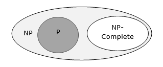
If a polynomial time algorithm exists for any of these problems, all problems in NP would be polynomial time solvable. These problems are called NP-complete. The phenomenon of NP-completeness is important for both theoretical and practical reasons.

Definition of NP-Completeness

A language B is NP-complete if it satisfies two conditions

• B is in NP
• Every A in NP is polynomial time reducible to B.

If a language satisfies the second property, but not necessarily the first one, the language B is known as NP-Hard. Informally, a search problem B is NP-Hard if there exists some NP-Complete problem A that Turing reduces to B.

The problem in NP-Hard cannot be solved in polynomial time, until P = NP. If a problem is proved to be NPC, there is no need to waste time on trying to find an efficient algorithm for it. Instead, we can focus on design approximation algorithm.

NP-Complete Problems

Following are some NP-Complete problems, for which no polynomial time algorithm is known.

• Determining whether a graph has a Hamiltonian cycle
• Determining whether a Boolean formula is satisfiable, etc.

Explore our latest online courses and learn new skills at your own pace. Enroll and become a certified expert to boost your career.

NP-Hard Problems

The following problems are NP-Hard

• The circuit-satisfiability problem
• Set Cover
• Vertex Cover
• Travelling Salesman Problem

In this context, now we will discuss TSP is NP-Complete

TSP is NP-Complete

The traveling salesman problem consists of a salesman and a set of cities. The salesman has to visit each one of the cities starting from a certain one and returning to the same city. The challenge of the problem is that the traveling salesman wants to minimize the total length of the trip

Proof

To prove TSP is NP-Complete, first we have to prove that TSP belongs to NP. In TSP, we find a tour and check that the tour contains each vertex once. Then the total cost of the edges of the tour is calculated. Finally, we check if the cost is minimum. This can be completed in polynomial time. Thus TSP belongs to NP.

Secondly, we have to prove that TSP is NP-hard. To prove this, one way is to show that Hamiltonian cycle ≤_p TSP (as we know that the Hamiltonian cycle problem is NPcomplete).

Assume G = (V, E) to be an instance of Hamiltonian cycle.

Hence, an instance of TSP is constructed. We create the complete graph G^‘ = (V, E^‘), where

Thus, the cost function is defined as follows −

Now, suppose that a Hamiltonian cycle h exists in G. It is clear that the cost of each edge in h is 0 in G^‘ as each edge belongs to E. Therefore, h has a cost of 0 in G^‘. Thus, if graph G has a Hamiltonian cycle, then graph G^‘ has a tour of 0 cost.

Conversely, we assume that G^‘ has a tour h^‘ of cost at most 0. The cost of edges in E^‘ are 0 and 1 by definition. Hence, each edge must have a cost of 0 as the cost of h^‘ is 0. We therefore conclude that h^‘ contains only edges in E.

We have thus proven that G has a Hamiltonian cycle, if and only if G^‘ has a tour of cost at most 0. TSP is NP-complete.

 

Travelling Salesman Problem (Greedy Approach)

The travelling salesman problem is a graph computational problem where the salesman needs to visit all cities (represented using nodes in a graph) in a list just once and the distances (represented using edges in the graph) between all these cities are known. The solution that is needed to be found for this problem is the shortest possible route in which the salesman visits all the cities and returns to the origin city.

If you look at the graph below, considering that the salesman starts from the vertex ‘a’, they need to travel through all the remaining vertices b, c, d, e, f and get back to ‘a’ while making sure that the cost taken is minimum.

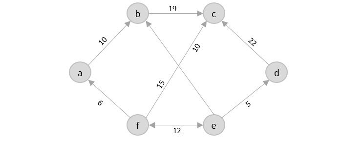
There are various approaches to find the solution to the travelling salesman problem: naive approach, greedy approach, dynamic programming approach, etc. In this tutorial we will be learning about solving travelling salesman problem using greedy approach.

Travelling Salesperson Algorithm

As the definition for greedy approach states, we need to find the best optimal solution locally to figure out the global optimal solution. The inputs taken by the algorithm are the graph G {V, E}, where V is the set of vertices and E is the set of edges. The shortest path of graph G starting from one vertex returning to the same vertex is obtained as the output.

Algorithm

• Travelling salesman problem takes a graph G {V, E} as an input and declare another graph as the output (say G’) which will record the path the salesman is going to take from one node to another.
• The algorithm begins by sorting all the edges in the input graph G from the least distance to the largest distance.
• The first edge selected is the edge with least distance, and one of the two vertices (say A and B) being the origin node (say A).
• Then among the adjacent edges of the node other than the origin node (B), find the least cost edge and add it onto the output graph.
• Continue the process with further nodes making sure there are no cycles in the output graph and the path reaches back to the origin node A.
• However, if the origin is mentioned in the given problem, then the solution must always start from that node only. Let us look at some example problems to understand this better.

Examples

Consider the following graph with six cities and the distances between them −

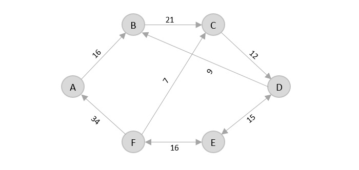
From the given graph, since the origin is already mentioned, the solution must always start from that node. Among the edges leading from A, A → B has the shortest distance.

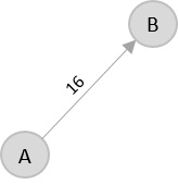
Then, B → C has the shortest and only edge between, therefore it is included in the output graph.

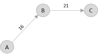
There’s only one edge between C → D, therefore it is added to the output graph.

There’s two outward edges from D. Even though, D → B has lower distance than D → E, B is already visited once and it would form a cycle if added to the output graph. Therefore, D → E is added into the output graph.

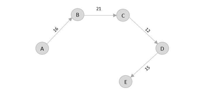
There’s only one edge from e, that is E → F. Therefore, it is added into the output graph.

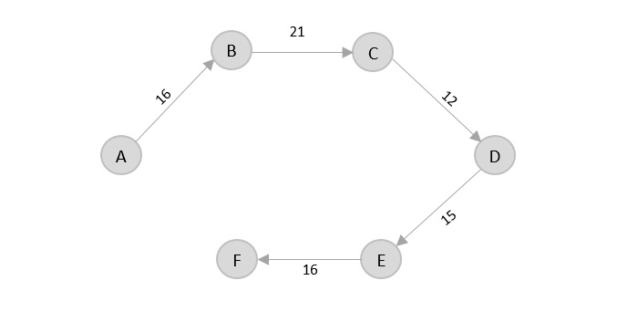
Again, even though F → C has lower distance than F → A, F → A is added into the output graph in order to avoid the cycle that would form and C is already visited once.

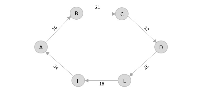
The shortest path that originates and ends at A is A → B → C → D → E → F → A

The cost of the path is: 16 + 21 + 12 + 15 + 16 + 34 = 114.

Even though, the cost of path could be decreased if it originates from other nodes but the question is not raised with respect to that.